2D Linear Inversion of Crosswell Tomography Data¶

import numpy as np
from geoscilabs.inversion.TomographyInversion import TomographyInversionApp
import matplotlib.pyplot as plt
from ipywidgets import interact, IntSlider
%matplotlib inline

Purpose¶

From the Linear inversion notebook (1D), we learned important apsects about the linear inversion. However, real world geophysical inverse problem are not often 1D, but multidimensional (2D or 3D), and this extension of dimension allows us to put more apriori (or geologic) information through the regularization term. In this notebook, we explore these multidimensional aspects of the linear inversion by using 2D traveltime croswell tomography example.

Outline¶

This notebook includes three steps:

Step 1: Generate a velocity model
Step 2: Simulate traveltime data and add noise
Step 3: Run $l_2$ inversion

Step 1: Generate a velocity model¶

Here we set up a velocity model using a following app. Controlling parameters of the app are:

set mesh: use active only when you want to change the 2D mesh
add block: use active when you want to add block (if not stay inactive)
model type: background or block
show grid?: show grid of the mesh
v0: velocity of the background
v1: velocity of the block
xc: x center of the block
yc: y center of the block
dx: width of the block
dz: thickness of the block
nx: # of cells in x-direction (this is only active when set_mesh=active)
ny: # of cells in y-direction (this is only active when set_mesh=active)

Re-running the following cell will reset the app to the default parameters.

Changing # of cells in $x$ - or $z$ - direction¶

Adjustable parameters: set mesh, nx, ny

The 2D domain is fixed at 200m × 400m. The number of cells in each direction can be changed which alters the size of cells in each direction. To change either nx or ny:

Set set mesh=active. This will change the view to the background model v0.
Adjust nx and or ny using the sliders. The size of the cells is diplayed above the model.
When finished adjusting the mesh set set mesh=inactive.

Changing the background model¶

Adjustable parameters: model type, v0

To change the value of the constant background velocity model:

Set model type=background. This will change the view to the background model v0.
Adjust v0 using the slider.
When finished ajusting set model type=block

Changing the parameters of a single block¶

Adjustable parameters: add block, model type, v1, xc, zc, dx, dz

To change the parameters of a single block model (default):

Set add block=active.
Adjust v1, xc, zc, dx, dz using the sliders. The original block settings will remain in view.
When finished ajusting set model type=background
To confirm the parameter changes and veiw the current block, set model type=block

Adding more blocks¶

Adjustable parameters: add block, v1, xc, zc, dx, dz

The model can contain multiple blocks. To add new blocks to the model:

Set add block=inactive
Adjust the parameters of the new block v1, xc, zc, dx, dz. The velocity model will not change yet. The white boundary of the new block serves as a preview.
When finished adjusting the new block parameters set add block=active. The velocity model will be updated with the new block.
Repeat Steps 1-3 to add more blocks.

The parameters of the blocks in a multi-block model cannot be changed once the block has been added. Attempting to adjust the parameters after the block has been added to the model (following the directions in the previous section “Changing the parameters of a single block”) will remove all previous blocks. A single block model with the current block is created.

app = TomographyInversionApp()
app.interact_plot_model()

Step 2: Simulate travel time data and add noise¶

Within this app, by using the velocity model set up above, we simulate traveltime tomography data and add Gaussian noise. This syntehtic data set will be used in the following inversion module. Controlling parameters are:

percent (%): percentage of the Gaussian noise
floor (s): floor of the Gaussain noise
random seed: seed to generate random variables having normal distribution
tx_rx_plane or histogram: data display options
update: this buttion is for the interaction with the Step 1 app. If the velocity model is changed by altering the first app, you can simply click update to run simulation again with the updated velocity model.

app.interact_data()

Step 3: $l_2$ inversion¶

Here we invert the data generated in Step 2 and explore the results. Step 3 is divided into four sections:

Step 3.1: Run inversion
Step 3.2: Plot recovered model
Step 3.3: Plot predicted data
Step 3.4: Plot misfit curves

Step 3.1: Run inversion¶

The inversion, run in the cell below, requires the following input parameters, each of which can be adjusted:

maxIter: maximum number of iterations
m0: initial model
mref: reference model
percentage: percent standard deviation for the uncertainty
floor: floor value for the uncertainty
chifact: chifactor for the target misfit
beta0_ratio: ratio to set the initial beta
coolingFactor: cooling factor to cool beta
n_iter_per_beta: # of interations for each beta value
alpha_s: $\alpha_s$
alpha_x: $\alpha_x$
alpha_z: $\alpha_z$
use_target: use target misfit as a stopping criteria or not

model, pred, save = app.run_inversion(
    maxIter=20,
    m0=1./1000.,
    mref=1./1000.,
    percentage=0,
    floor=0.01,
    chifact=0.1,
    beta0_ratio=1e2,
    coolingFactor=2,
    n_iter_per_beta=1,
    alpha_s=1/(app.mesh_prop.hx.min())**2,
    alpha_x=1,
    alpha_z=1,
    use_target=True
)

0.1

        SimPEG.InvProblem is setting bfgsH0 to the inverse of the eval2Deriv.
        ***Done using same Solver and solverOpts as the problem***
SimPEG.SaveOutputEveryIteration will save your inversion progress as: '###-InversionModel-2021-03-11-21-26.txt'
model has any nan: 0
=============================== Projected GNCG ===============================
  #     beta     phi_d     phi_m       f      |proj(x-g)-x|  LS    Comment   
-----------------------------------------------------------------------------
x0 has any nan: 0
   0  1.59e+07  3.40e+02  0.00e+00  3.40e+02    1.12e+04      0              
   1  7.97e+06  1.47e+02  1.07e-06  1.56e+02    4.92e+04      0              
   2  3.98e+06  1.33e+02  2.36e-06  1.42e+02    4.72e+04      0   Skip BFGS  
   3  1.99e+06  1.16e+02  5.55e-06  1.27e+02    4.31e+04      0   Skip BFGS  
   4  9.96e+05  9.70e+01  1.23e-05  1.09e+02    3.79e+04      0   Skip BFGS  
   5  4.98e+05  7.91e+01  2.51e-05  9.17e+01    3.24e+04      0   Skip BFGS  
   6  2.49e+05  6.27e+01  4.89e-05  7.49e+01    2.67e+04      0   Skip BFGS  
   7  1.24e+05  4.85e+01  8.96e-05  5.96e+01    2.10e+04      0   Skip BFGS  
   8  6.22e+04  3.73e+01  1.53e-04  4.68e+01    1.61e+04      0   Skip BFGS  
   9  3.11e+04  2.87e+01  2.52e-04  3.65e+01    1.24e+04      0   Skip BFGS  
  10  1.56e+04  2.14e+01  4.18e-04  2.79e+01    9.50e+03      0   Skip BFGS  
  11  7.78e+03  1.51e+01  7.09e-04  2.06e+01    7.05e+03      0   Skip BFGS  
  12  3.89e+03  1.00e+01  1.17e-03  1.46e+01    5.21e+03      0   Skip BFGS  
  13  1.94e+03  6.53e+00  1.80e-03  1.00e+01    3.32e+03      0   Skip BFGS  
------------------------- STOP! -------------------------
1 : |fc-fOld| = 0.0000e+00 <= tolF*(1+|f0|) = 3.4119e+01
1 : |xc-x_last| = 3.0710e-04 <= tolX*(1+|x0|) = 1.0141e-01
0 : |proj(x-g)-x|    = 3.3180e+03 <= tolG          = 1.0000e-10
0 : |proj(x-g)-x|    = 3.3180e+03 <= 1e3*eps       = 1.0000e-07
0 : maxIter   =      20    <= iter          =     14
------------------------- DONE! -------------------------

Step 3.2: Plot recovered model¶

The app below displays the:

Recovered model from the inversion in Step 3.1 (left)
True model generated in Step 1 (right)

The model view is changed using:

ii: each iteration of the inversion (ii=0 is the initial model m0)
fixed: when selected the colorbar of both plots have the same fixed limits

app.interact_model_inversion(model, clim=None)

Step 3.3: Plot predicted data¶

The app below displays the:

Obversed data calculated in Step 2 (left)
Predicted data from the inversion in Step 3.1 (center)
Normalized misfit between the observed and predicted data (right)

The predicted data and normalized misfit view is changed using:

ii: each iteration of the inversion (ii=0 is the initial model m0)
fixed: when selected the colorbar of both data plots have the same fixed limits

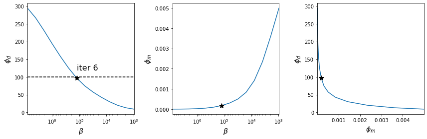
app.interact_data_inversion(pred)

Step 3.4: Plot misfit curves¶

Plot of the data misfit and model norm values as functions of inversion iteration
Tikhonov curves with the optimal values indicated by the star
1. Data misfit as a function of trade-off parameter β
2. Model norm as a function of trade-off parameter β
3. Data misfit versus model norm