Forward simulation of TDEM on cylindrical meshes with SimPEG
In this notebook, we demonstrate a time domain electromagnetic simulation using SimPEG. We use a cylindrically symmetric mesh and simulate a sounding over a sphere in a halfspace.
# packages from the python ecosystem
import numpy as np
import matplotlib.pyplot as plt
from matplotlib.colors import LogNorm, Normalize
import ipywidgets
from scipy.constants import mu_0

# software from the SimPEG ecosystem
import discretize
from SimPEG import maps
from SimPEG.electromagnetics import time_domain as tdem
from pymatsolver import Pardiso
# set a bigger font size
from matplotlib import rcParams
rcParams["font.size"]=14Define model parameters
# electrical conductivities in S/m
sig_halfspace = 1e-3
sig_sphere = 1e-1
sig_air = 1e-8
# depth to center, radius in m
sphere_z = -50.
sphere_radius = 30.Survey parameters
# coincident source-receiver
src_height = 30.
rx_offset = 0.

# times when the receiver will sample db/dt
times = np.logspace(-6, -3, 30)

# source and receiver location in 3D space
src_loc = np.r_[0., 0., src_height]
rx_loc = np.atleast_2d(np.r_[rx_offset, 0., src_height])
# print the min and max diffusion distances to make sure mesh is
# fine enough and extends far enough
def diffusion_distance(sigma, time):
return 1.28*np.sqrt(time/(sigma * mu_0))
print(f'max diffusion distance: {diffusion_distance(sig_halfspace, times.max()):0.2e} m')max diffusion distance: 1.14e+03 m
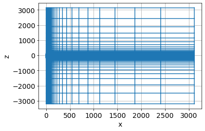
Create a mesh
Up until now, we have just been working with standard python libraries. Now, we will create a cylindrically symmetric mesh on which we will perform the simulation. Note that for an EM experiment, we need the mesh to extend sufficiently far (well beyond the diffusion distance) to ensure the boundary condutions are satisfied
# x-direction
csx = 1  # core mesh cell width in the x-direction
ncx = np.ceil(2*sphere_radius/csx)  # number of core x-cells
npadx = 25  # number of x padding cells

# z-direction
csz = 1  # core mesh cell width in the z-direction
ncz = np.ceil(2*(src_height - (sphere_z-sphere_radius))/csz) # number of core z-cells
npadz = 25  # number of z padding cells

# padding factor (expand cells to infinity)
pf = 1.3
# cell spacings in the x and z directions
hx = discretize.utils.unpack_widths([(csx, ncx), (csx, npadx, pf)])
hz = discretize.utils.unpack_widths([(csz, npadz, -pf), (csz, ncz), (csz, npadz, pf)])
# define a mesh
mesh = discretize.CylMesh([hx, 1, hz], origin=np.r_[0.,0., -hz.sum()/2.-src_height])
mesh.plot_grid();
print(mesh.nC)22950
put the model on the mesh
# create a vector that has one entry for every cell center
sigma = sig_air*np.ones(mesh.nC)  # start by defining the conductivity of the air everwhere
sigma[mesh.gridCC[:,2] < 0.] = sig_halfspace  # assign halfspace cells below the earth

sigma_background = sigma.copy()

# indices of the sphere (where (x-x0)**2 + (z-z0)**2 <= R**2)
sphere_ind = (mesh.gridCC[:,0]**2 + (mesh.gridCC[:,2] - sphere_z)**2) <= sphere_radius**2
sigma[sphere_ind] = sig_sphere  # assign the conductivity of the sphere
fig, ax = plt.subplots(1,1)
cb = plt.colorbar(mesh.plotImage(np.log10(sigma), ax=ax, mirror=True)[0])
# plot formatting and titles
cb.set_label('$\log_{10}\sigma$', fontsize=13)
ax.axis('equal')
ax.set_xlim([-120., 120.])
ax.set_ylim([-100., 30.])
ax.set_title('Conductivity Model');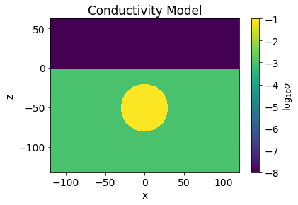
create the survey
A SimPEG survey needs to know about the sources and receivers. First, we define the receivers (in this case, a single receiver that is coincident with the source.)
# Define the receivers
dbdt_z = tdem.receivers.Point_dbdt(locs=rx_loc, times=times, orientation='z')  # vertical db_dt
# Define the list of sources - one source for each frequency. The source is a point dipole oriented
# in the z-direction
source_list = [
tdem.sources.CircularLoop(
receiver_list=[dbdt_z], radius=1, location=src_loc, orientation='z', waveform=tdem.sources.StepOffWaveform()
)
]
survey = tdem.Survey(source_list)set up a simulation
# solve the problem at these times
nsteps = 20
dt_list = [1e-8, 3e-8, 1e-7, 3e-7, 1e-6, 3e-6, 1e-5, 3e-5, 1e-4]
time_steps = [(dt, nsteps) for dt in dt_list]

simulation = tdem.Simulation3DElectricField(
    mesh, time_steps=time_steps, survey=survey,
    solver=Pardiso, sigmaMap=maps.IdentityMap(mesh)
)
%%time
print('solving with sphere ... ')
fields = simulation.fields(sigma)
print('... done ')solving with sphere ...
... done
CPU times: user 19.1 s, sys: 946 ms, total: 20.1 s
Wall time: 5.28 s
%%time
print('solving without sphere ... ')
fields_background = simulation.fields(sigma_background)
print('... done ')
solving without sphere ...
... done
CPU times: user 18.6 s, sys: 871 ms, total: 19.5 s
Wall time: 5.04 s
define some utility functions for plotting
def plot_field(model="background", view="dbdt", time_ind=1, ax=None):
    min_field, max_field = None, None
    vType = "CC"
    view_type="real"
    mirror_data=None

    if ax is None:
        fig, ax = plt.subplots(1,1, figsize=(8,5))

    if view in ["j", "dbdt"]:
        if model == "background":
            plotme = fields_background[source_list, view, time_ind]
        else:
            plotme = fields[source_list, view, time_ind]
        max_field = np.abs(plotme).max() #use to set colorbar limits

        if view == "dbdt":
            vType, view_type="F", "vec"
            cb_range = 5e2  # dynamic range of colorbar
            min_field = max_field/cb_range
            norm=LogNorm(vmin=min_field, vmax=max_field)
        elif view == "j":
            plotme = mesh.average_edge_y_to_cell * plotme
            mirror_data = -plotme
            norm=Normalize(vmin=-max_field, vmax=max_field)
    else:
        label = "$\sigma$"
        norm=LogNorm(vmin=sig_air, vmax=np.max([sig_sphere, sig_halfspace]))
        if model == "background":
            plotme = sigma_background
        else:
            plotme = sigma

    cb = plt.colorbar(mesh.plotImage(
        plotme,
        vType=vType, view=view_type, mirror_data=mirror_data,
        range_x=[-150., 150.], range_y=[-150., 70.],
        pcolorOpts={'norm': norm}, streamOpts={'color': 'w'},
        stream_threshold=min_field, mirror=True, ax=ax,
    )[0], ax=ax)
    cb.set_label(view)


def plot_sphere_outline(ax):
    x = np.linspace(-sphere_radius, sphere_radius, 100)
    ax.plot(x, np.sqrt(sphere_radius**2 - x**2) + sphere_z, color='k', alpha=0.5, lw=0.5)
    ax.plot(x, -np.sqrt(sphere_radius**2 - x**2) + sphere_z, color='k', alpha=0.5, lw=0.5)
def plot_fields_sphere(model="background", view="dbdt", time_ind=1):
fig, ax = plt.subplots(1,1, figsize=(8,5))
plot_field(model, view, time_ind, ax)
# plot the outline of the sphere
if model == "sphere":
plot_sphere_outline(ax)
# plot the source locations and earth surface
ax.plot(src_loc[0],src_loc[2],'C1o', markersize=6)
ax.plot(np.r_[-200, 200], np.r_[0., 0.], 'w:')
# give it a title
ax.set_title(f'{view}, {simulation.times[time_ind]*1e3:10.2e} ms')
ax.set_aspect(1)
# return axView the simulated fields
ipywidgets.interact(
    plot_fields_sphere,
    model=ipywidgets.ToggleButtons(options=["background", "sphere"], value="background"),
    view=ipywidgets.ToggleButtons(options=["model", "j", "dbdt"], value="model"),
    time_ind=ipywidgets.IntSlider(min=1, max=len(simulation.time_steps)-1, value=1, continuous_update=False),
);
Loading...
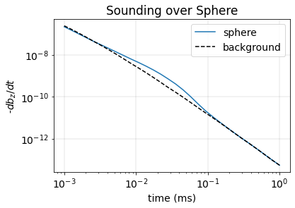
predicted data
dpred = simulation.dpred(sigma, f=fields)
dpred_background = simulation.dpred(sigma_background, f=fields_background)
# Plot
fig, ax = plt.subplots(1,1)
ax.loglog(1e3*times, -dpred, label="sphere")
ax.loglog(1e3*times, -dpred_background, '--k', label="background")
ax.grid(True, color='k',linestyle="-", linewidth=0.1)
ax.legend()
ax.set_title('Sounding over Sphere')
ax.set_ylabel('-$db_z/dt$')
ax.set_xlabel('time (ms)');