Data Misfit
The observations encode our knowledge about the model obtained from the survey. Any candidate solution must produce simulated (or predicted) data that “fit” the observations. Central to this goal is the choice of a “criterion” for measuring misfit between observed and predicted data, and a “tolerance” for deciding what value constitutes an acceptable fit. This is a subject on which an enormous amount of literature has been written but a good reference, written for the inverse problem, is Parker (1994). When errors are Gaussian with zero mean and known standard deviation, then the -norm, is an appropriate choice. We define the misfit to be
where is the observation, is its estimated standard deviation, and is the predicted datum. The quantity
is a random variable with zero mean and unit standard deviation and , which is the sum of squares of these variables, is the well known statistical variable. It has an expected value ((3)) and variance ((4)).
Thus if we are attempting to find a model that acceptably fits the data, then models with are good candidates. For many problems we often denote a target misfit to be
but this must only be regarded as a reasonable estimate and some flexibility should be entertained.
In times past, it was felt that getting an acceptable fit to the data was a sufficient criterion for having a successful inversion. The observed data are inverted to produce a model , which is used to forward model the predicted data . The observed and predicted data are then compared using the data misfit measure. If the model is accepted, but if not, the inversion parameters are adjusted and the process is repeated until an acceptable model is reached. The workflow procedure is delineated below.
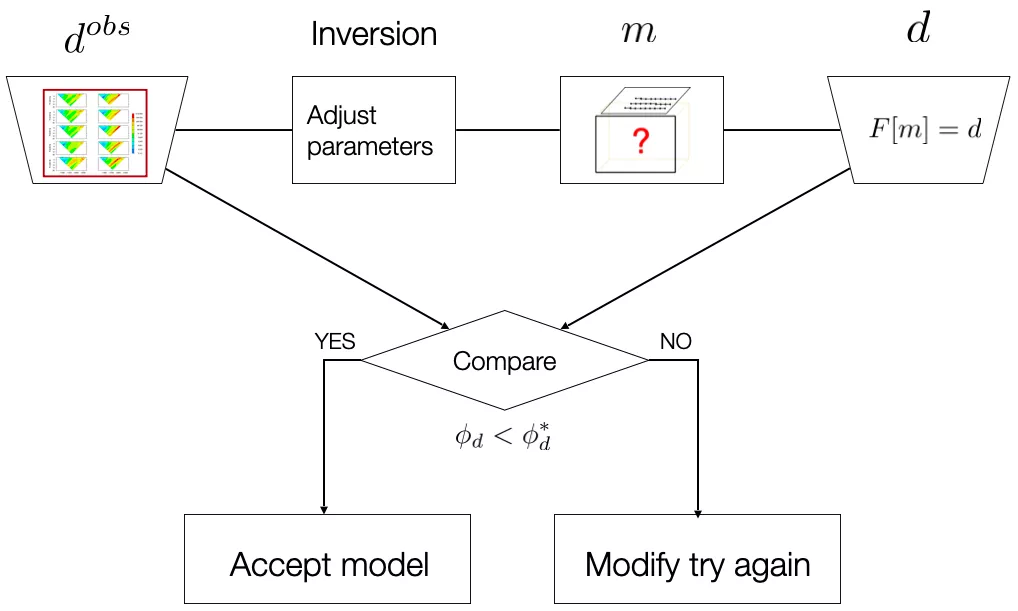
Finding a model that fits the data is a necessary component of an inversion algorithm, but as shown in the next section, it is not sufficient.
- Parker, R. L. (1994). Geophysical Inverse Theory (Vol. 1). Princeton University Press. 10.2307/j.ctvs32s89