Linear Tikhonov Inversion

Introduction¶

In this chapter we present the basic elements for how an inverse problem can be formulated and solved using optimization theory. The quantity to be minimized is a weighted sum of misfit and regularization terms with their relative importance controlled by an adjustable Tikhonov parameter.

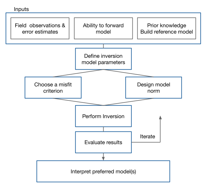
The inverse problem has many elements and a solution is best achieved by adhering to the workflow shown in Figure 1 below. Throughout this chapter we investigate each of these steps and illustrate the concepts with a simple linear problem. Jupyter notebooks are provided so that the concepts can be explored (LinearTikhonovInversion_App.ipynb) and all the corresponding figures in this article can be reproduced using LinearTikhonovInversion_Notebook.ipynb. The formative material for this chapter is extracted from the tutorial paper Inversion for Applied Geophysics: A Tutorial Oldenburg & Li, 2005.

Key Points

• Forward Problem - model, mesh, kernel function, data, noise
• Inverse Problem - data misfit, regularization function, norms
• Optimization - choice of Tikhonov parameter

Contents¶

2.1. Forward Problem: Defining the model, kernel function, data and noise for the forward problem. We also define the mesh, model parameters and mapping for discrete forward problems that can be solved numerically.

2.2. Defining the Inverse Problem:

2.3. Data Misfit:

2.4. Non-Uniquness:

2.5. Model Norm:

2.6. Objective Function:

2.7. Summary: An overview of what was learned in this chapter.