Forward Problem

For a linear system, the forward problem ((2)) can often be represented in the form of an integral equation (technically a Fredholm equation of the Second kind) as shown below.

The model $m(x)$ is a function defined on the closed region $[a,b]$, and $g_j(x)$ is the kernel function which encapsulates the physics of the problem. The datum, $d_j$ is the inner product of the kernel and the model. It is sometimes helpful to think of the kernel as the “window” through which a model is viewed. In this section we will step through the essential details for carrying out the forward modelling. We first design a model, introduce a “mesh” to discretize it, discretize the kernels and form sensitivities, generate the data through a matrix vector multiplication and then add noise. These data will then be inverted.

For our synthetic problem, we start by creating the function that we will later want to retrieve with the inversion. The model can be any function but here we combine a background, box car, and a Gaussian; the domain will be [0,1], shown in Figure A.

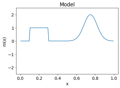
Figure A: Default model from the corresponding inversion application. The model combines a background value with box car and Gaussian functions on the domain [0,1]. LinearTikhonovInversion_Notebook.ipynb

2.3.1. Mesh¶

In our next step we design a mesh on which our model is defined and on which all of the numerical computations are carried. We discretize our domain into $M$ cells of uniform thickness. If we think about the “x-direction” as being depth, then this discretization would be like having a layered earth.

Our “model” is now an M-length vector $\mathbf m = (m_1, m_2, …, m_M)$. In fact, the function plotted in Figure A has already been discretized.

2.3.2. Kernels and Data¶

Our goal is to carry out an experiment that produces data that are sensitive to the model shown in Figure A. For our linear system ((1)) this means choosing the kernel functions. In reality, these kernel functions are controlled by the governing physical equations and the specifics of the sources and receivers for the experiment. For our investigation we select oscillatory functions which decay with depth. These are chosen because they are mathematically easy to manipulate and they also have a connection with many geophysical surveys, for example, in a frequency domain electromagnetic survey a sinusoidal wave propagates into the earth and continually decays as energy is dissipated. The kernel $g_j(x)$ corresponding to $d_j$ is given by

Thus $p_j$ controls the rate of decay of the kernel and $q_j$ controls the frequency; the kernel will undergo $q_j$ complete cycles in the domain [0,1]. In our example, each of the ranges $[p_{min}, p_{max}]$ and $[q_{min}, q_{max}]$ is divided into M intervals but this is only for convenience. In principle these numbers can be arbitrarily specified. As an example the image below displays three kernels produced with $q = [1, 2, 3]$ and $p = [0, 1, 2]$. Note the successive decrease in amplitude at $x=1.0$.

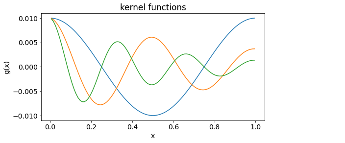
Figure B: Example of three kernels ((2)) for the app where q=[1,2,3] and p=[0,1,2]. LinearTikhonovInversion_Notebook.ipynb

To simulate the data we need to evaluate (1). The model has been discretized with the 1D mesh. The expression for the data becomes

where $\mathbf g_j$ is now referred to as a sensitivity kernel. When the discretization is uniform, the only difference between the kernel $g_j(x)$ and the sensitivity $\mathbf g_j$ is a scaling factor that is equal to the discretization width. However, for nonuniform meshes these quantities can look quite different, and confusing kernels and sensitivities, can lead to unintended consequences in an inversion. We shall make this distinction clear at the outset.

To expand the above to deal with $N$ data. We define a sensitivity matrix $\mathbf{G}$. The $j^{th}$ row of $\mathbf{G}$ is formed by $\mathbf g_j$ so $\mathbf{d}$ looks like

where the individual elements of $G$ are

$\mathbf{G}$ is an $N \times M$ matrix ($N$ data and $M$ model elements). Using the model in Figure A and our sensitivity matrix $\mathbf{G}$ we forward model the data. The model, rows of the sensitivity matrix, and corresponding data are shown in Figure C. The data are considered “clean” or “true” because they do not contain noise.

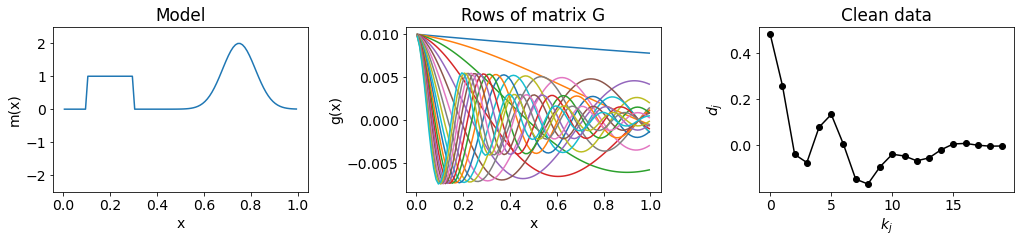
Figure C: Default display from the app of the model, rows (sensitivity kernels) of the matrix $\mathbf{G}$, and clean data. LinearTikhonovInversion_Notebook.ipynb

2.3.3. Adding Noise¶

Until now, we have only calculated the data $\mathbf{d}$, but observed data $\mathbf{d}^{obs}$ contain additive noise,

Throughout our work, the noise for a datum $d_j$ is assumed to be a realization of a Gaussian random variable with zero mean and standard deviation

this is a percentage of the datum plus a floor. The reason for this choice is as follows. In every experiment there is a base-level of noise due to instrument precision and other factors such as wind noise or ground vibrations. This can be represented as a Gaussian random variable with zero mean and standard deviation $\nu_j$ and a single value might be applicable for all of the data in the survey. This is often when the data do not have a large dynamic range such as might be found in gravity or magnetic data. In other cases the data can have a large dynamic range, such as in DC resistivity surveys or time domain EM data. To capture uncertainties in the data, a percentage value is more appropriate. If data range from 1.0 to $1e-4$ then a standard deviation of $10 \%$ of the smallest datum is likely an under-estimate for the datum that has unit amplitude.

These are important concepts and we’ll revisit them in more detail later. For now it suffices that “noise” can be added to the data according to (6). Here we choose $\epsilon_j = 0.03$. An example of the clean (true) data, a realization of the noise, and the noisy data are shown in Figure D. The error bars are superposed on the noisy data.

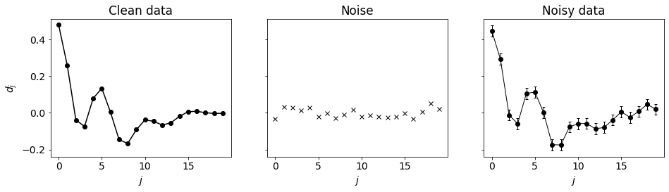
Figure D: Display of the clean data from Figure 2.5 with the added noise to create the noisy data. LinearTikhonovInversion_Notebook.ipynb

The construction of the forward problem for the 1D synthetic example provided many of the elements needed for the inverse problem. We have observed data, an estimate of the uncertainty within the data, the ability to forward model and we have discretized our problem. Our goal is to find the model that gave rise to the data. Within the context of our flow chart in 2.2. Defining the Inverse Problem-Figure 1 the next two items to address are the misfit criterion and model norm. We first address the issue of data misfit.