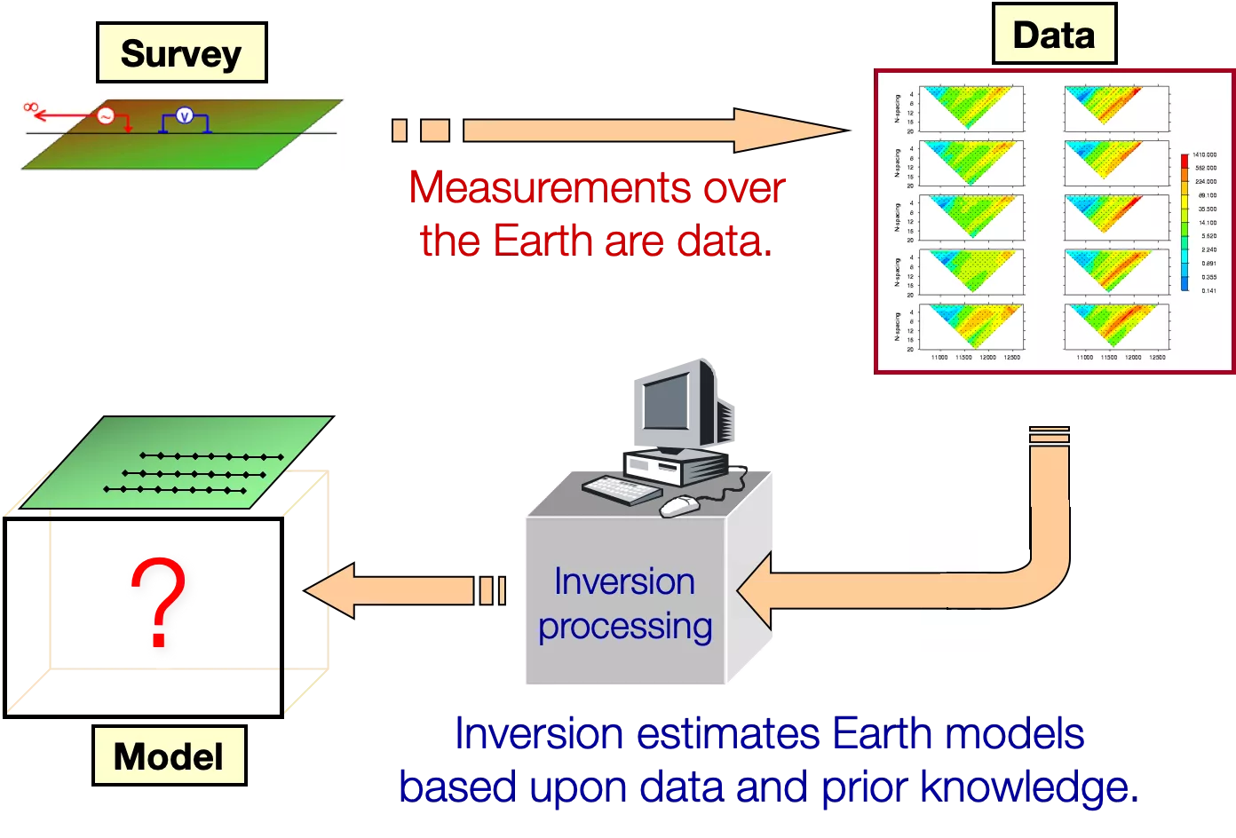
Introduction to Inversion

Occasionally it is possible to infer useful information directly by looking at the data map. For instance, when a target body is situated in a homogeneous background, the data might indicate an anomaly that could be inferred to be a sought structure. Historically, many mineral deposits have been drilled on this type of analysis. In general however, this approach produces unsatisfactory results. A more responsible way to proceed is to implement a procedure to “invert” the data and find the physical property model that gave rise to the observations. The ideal procedure is illustrated in Figure 1 below.

In reality we have only a finite number of observations and they are inaccurate. On the other hand the earth can be exceedingly complicated and so it might be anticipated that the simple ideas in the figure can be easily achieved. The next sections are devoted to understanding the fundamental challenges of inversion, namely origins of the nonuniqueness in the solution. We use some simple problems in seismology to illuminate this understanding and help define our forward and inverse mappings as well as the lexicon we shall use throughout these chapters.

1.3.1. Seismic Refraction Experiment¶

A common geophysical experiment that captures some of the essential ideas regarding an inverse problem is the seismic refraction survey. We consider a 1D earth in which the velocity increases with depth. Energy from a source propagates into the earth but continually refracts according to Snell’s law. It turns surface-ward at a critical point and returns to the surface where it can be recorded by a seismometer. The ray path in Figure 2 shows how the energy travels.

If $x_j$ denotes the receiver location then the suite of seismograms at the associate receivers looks like that in Figure 3.

The time of the onset of the energy is of interest here; this is indicated as $t_j$ in the plot (Figure 4). This value is equal to the integral of the slowness along the ray path. There is always uncertainty in picking these first arrivals because the arrivals don’t have a sharp onset and there is background noise on the seismic record. The data, along with estimated uncertainties, are plotted in the diagram below (Figure 4).

1.3.2. Inverse problem¶

The inverse problem can be articulated as: “Given the survey information, data $d_j^{obs}$ (j=1,N), and an estimate of the uncertainty for each datum, what is the earth model, in this case the velocity structure $v(z)$, that produced these data?” An important component in addressing the inverse problem is that we have the capability to carry out a forward modelling. For this problem, for a given $v(z)$, how can we simulate the travel times.