Inverse Problem Fundamental Challenges
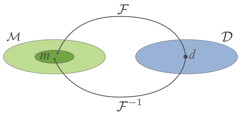
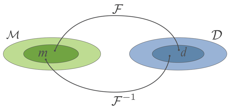
Inversion is the process of mapping from the data space to the model space , shown in Figure 1.
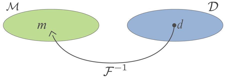
Figure 1:Inversion is the process of mapping from the data space to the model space .
Two fundamental challenges when inverting data is the ill-conditioning of the problem and nonuniqueness of the solution. We can obtain intuition for this by considering the relationship in seismology between rms velocity and interval velocity originally presented in 1.3 Forward Mapping-(13). For this problem we define the following:
- Forward Problem : Given the model compute the data
- Inverse Problem : Given the data compute the model
Thus, given the data, , what is the velocity model, that produced the data? There are numerous questions that can be asked:
- Does a solution exist? - Is there any model that can produce the data?
- How do we construct a solution?
- Is the solution unique? - If you have found one candidate, are there others?
- How do we handle nonuniqueness? - If there are multiple solutions, which model best reflects the subsurface physical property distribution?
The answers to these questions depend on the available data and it’s insightful to consider the following cases
- infinite amount of accurate data (perfection ✨ )
- finite amount of accurate data (no noise 💯 )
- finite amount of inaccurate data (reality 🌎 )
- changes to the model due to a small perturbation of the data
In the forward problem we are given and we calculate “exactly” by carrying out the integration analytically ((1)) or numerically using extreme precision. The result is a function on the interval .
We notice that each datum is an integral of and hence structure observed in will appear as smoothed structure in the data . That is, the forward operator is a “smoother”. As an example consider an interval . The interval velocity model and data are shown below for the special case of xxxx
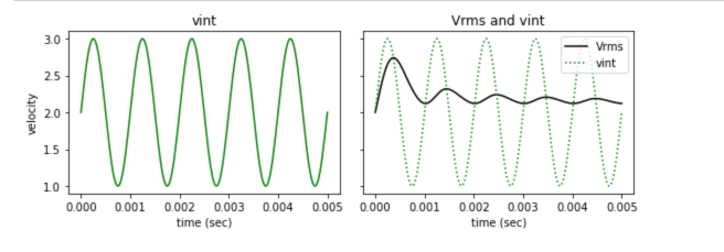
As a general rule all forward modelling operators are smoothers and the issue is conceptualized in the figure below
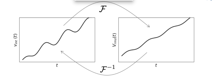
If the forward mapping F smooths, then the inverse operator F^-1must “roughen”. This is easily seen in our example where the analytic inverse
exists.
We notice that there is a time derivate of the data. Differentiation is a roughening operator. Moreover this derivative is multiplied by which means that small changes in the data at later times will produce large changes in . To explore the main concepts, we define an example for the rms velocity data,
where is a constant, the amplitude of the sinusoid, and the frequency in Hz. The corresponding derivative of the data, required for the analytic inverse calculation ((2)) is
We can solve equation (2) numerically by evaluating the integrand on a very fine mesh and using a quadrature integration and a finite difference for the derivative. The result is presented in Fig xx

The true and recovered interval velocity are identical.
1.5.1 Nonuniqueness
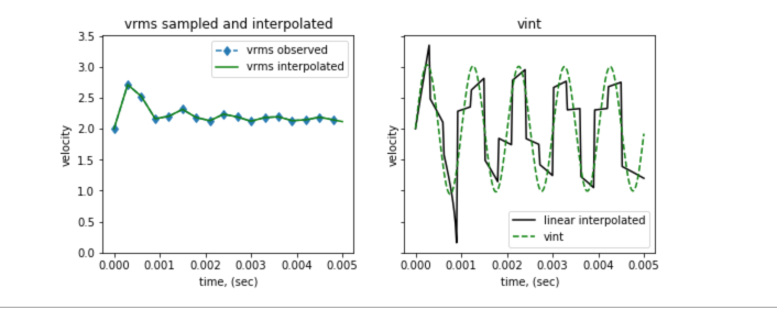
The above example illustrated the idealistic case where we have an infinite number of accurate data. We were able to recover the initial velocity model. We now explore the case where only a finite number of data exist. We do this by sampling at times , interpolate the data to obtain the function, as illustrated in the figure below.
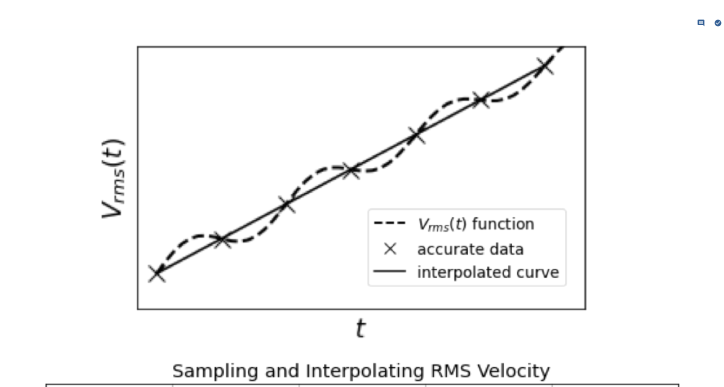
We then use the analytic formula (equation 2) to recover the interval velocity. The recovered model will depend upon the sampling and the interpolation scheme used.
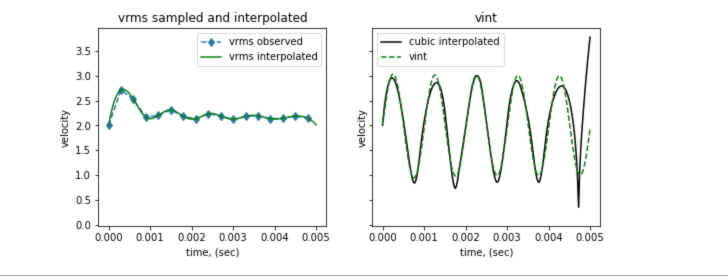
In the figure below we show the models recovered by using a linear and a cubic spline interpolation. At the scale plotted, the interpolated data are not greatly different but the cubic spline interpolated values are smoother and this is important when estimating a derivative of the data. The recovered velocities all show the five cycles in the mode but differ they from each other and also from the true model. Sine there are an infinite number of ways in which the finite number of data can be interpolated, the inverse problem is inherently non-unique.
Whereas in Figure 1 the application of maps to a single point in model space, with a finite number of data, we have many possible models; these are indicated by the dark green subspace of the model space in Figure 8.
The nonuniqueness is exacerbated when we have a finite number of data contaminated with noise. As shown in Figure %s below there are now more ways to interpolate the data and each interpolation will produce a different .
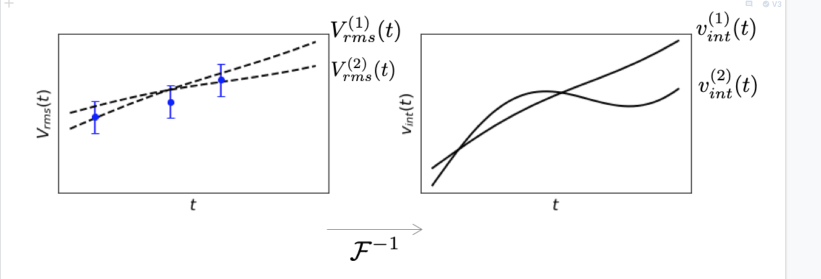
In the example below we add Gaussian noise with zero mean and standard deviation = 0.03 sec to the true data values. The point observations, along with error bars, are plotted in Fig xx. These data are linearly interpolated to generate for inversion. Even with small errors, the recovered model is exhibits considerable incorrect structure.
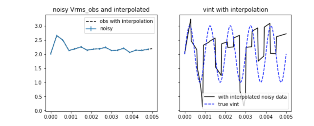
With respect to our mapping diagram, the inaccurate data to be inverted now populate the dark blue region of the data space and the inverse process maps to a larger, dark green, region of the model space (Figure 11).
1.5.2. Ill-conditioning
A second important aspect of the inverse problem is that of ill-conditioning. In most problems in geophysics, the forward operator is a smoothing operator. We saw that in the examples above but other insight arises from the fact that a geophysical datum often depends upon the physical properties in a volume of the subsurface. For instance, a gravity datum depends on the volumetric density distribution, or a DC potential depends upon all of the charges built up in the subsurface when a current is injected. So the data is effectively “averaging” the underlying physical property that we are attempting to find. The inverse problem must therefore “undo” this averaging. As in the previous examples, this often involves some type of differentiation of data to “roughen” the model. The practical question is whether that roughening results in model structures that are representative of the earth, or whether they present unrealistic structure. To quantify this we consider the following.
Let
where is a perturbation on the data. Let
where is the constructed model. We can then write
Suppose is small, does that mean is small? If it is not, then we will say that the problem is “ill-conditioned”.
Using the relationship between and in (2) suppose that our data is a constant, . The resulting model would be that same constant, . We can add a small sinusoidal perturbation to the data , such that the data is defined in (3). Despite the addition of small perturbation to the data, the resulting perturbation to the model is not small, as shown in (4), and thus
Therefore can be made arbitrarily large even if is small; we only need to increase the product . This inverse problem is considered ill-conditioned.