Solving an Ill-Posed Problem

The above work shows that the inverse problem is nonunique and ill-conditioned. This leads to the statement that “the inverse problem is ill-posed”. Any framework must handle these fundamental elements.

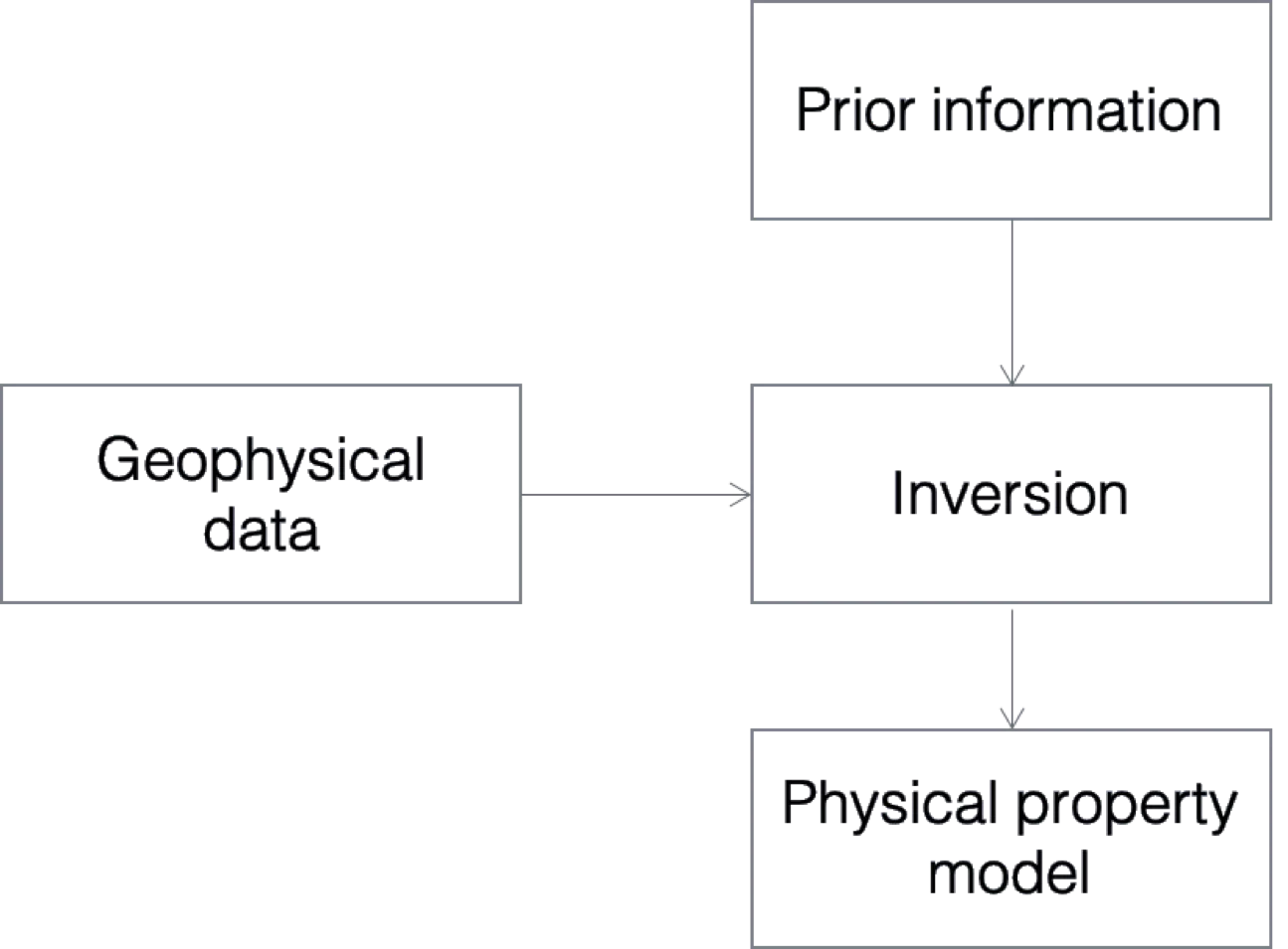
The major weapon for handling nonuniqueness is to add more information and find a model that satisfies the geophysical data as well as this a priori information. The simplified flow chart for the inversion is now shown in Figure 1.

The prior information takes many forms and throughout this module we will have opportunity to illustrate all of them. When thinking about a general geophysical inversion where we attempt to find a distribution of a physical property that can be translated into geology, we might have:

• General characteristics of the model - Is the geology expected to be smooth, discontinuous or compact?
• Geologic constraints - Knowledge about faults, overburden, rock units
• Reference model
• Bounds for the physical property
• Information from other geophysical surveys
• Expected rock units and physical property measurements.

The second issue of importance is the ill-conditioning of the inverse problem. The fundamental ill-conditioning is often automatically ameliorated by adding additional information into the problem. For instance, when adding a smallest model component into a Tikhonov inversion. However, there will always be ill-conditioning resulting from over-fitting noisy data and this needs to be addressed.

There are two general approaches to solving the inverse problem. The first is a probabilistic approach that rests on Bayesian analysis.

1.6.1. Bayesian (Probabilistic)¶

Use Bayes’ Theorem

where $P(m)$ is the prior information about $m$, $P(d^{obs}|m)$ is the probability about the data errors (likelihood), and $P(m|d^{obs})$ is the posterior probability for the model.

There are two pathways for analysis. The full Bayesian solution seeks to characterize
$P(m|d^{obs})$ and draw inferences from that distribution. The second is to find a particular solution that maximizes $P(m|d^{obs})$. This is call the maximum a posteriori (MAP) estimate.

Abundant resources for inversion using a Bayesian philosophy exist, but a classic is that of Tarantola (2005). We will have occasion towards the latter part of this module to work with a Bayesian formulation but most of our work will use the Tikhonov method.

1.6.2. Tikhonov (Deterministic)¶

In this approach the goal is to find a single “best” solution by solving an optimization problem:

where $\phi_d$ is the data misfit, $\phi_m$ is the regularization (model norm), β is the trade-off parameter, and $m_l, m_u$ are lower and upper bounds on the model. The constraints on the model from the geophysical information are embedded in the data misfit while the a priori information is encoded into the model norm and bounds.