Forward Mapping

Simulating data requires being able to solve

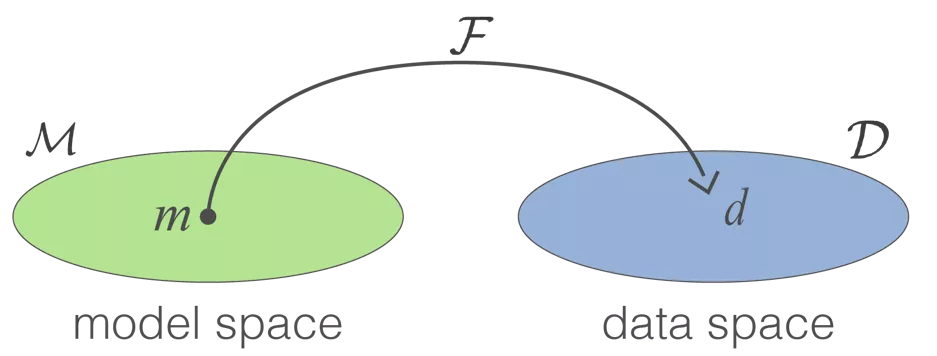
where $m$ is an element of the model space $\mathcal{M}$, and $\mathcal{F}$ is the forward mapping. $\mathcal{F}$ encompasses the physics of the problem, the geometry of the survey and details about Tx and Rx. The operation generates a simulated data set which is an element of data space $\mathcal{D}$. The procedure is conceptualized in the diagram below (Figure 1).

1.4.1. Model space¶

Model space is a vector space with key components. Its elements can be functions or Euclidean vectors. Model space comes equipped with two important attributes:

• Rules for inner products - This allows the concept of angles between elements to be computed. This allows us to determine whether elements are parallel or perpendicular to each other.
• Norms to measure length - In our optimization solution it will be important to measure the “length” of the vectors so that we can distinguish between small and large elements.

See Parker, 1994 for a more in depth discussion.

For our seismic refraction problem our model space elements can be functions $v(z)$ or $M$-length vector of velocity values: $\mathbf{v}=(v_1, \dots,v_M)$. These are shown in Figure 2.

1.4.2. Data Space¶

Observed data are generally a set of numbers and are consolidated into an elements of data space $\mathbf{d}=(d_1,\dots,d_N)~\in\R^N$. Each datum is calculated using

The subscript $j$ allows us to keep track of specifics for that datum, such as survey parameters, which field, etc.

1.4.3. Forward Mapping Operators¶

The forward mapping operator $\mathcal{F}$ is problem dependent and can be formulated as an integral or differential operator. Fundamentally however, it is useful to distinguish between two types: linear and nonlinear operators. Linear operators are the easiest to deal with in an inverse problem and understanding them forms a solid foundation for attacking nonlinear inverse problems.

1.4.3.1 Linear and Nonlinear Mappings¶

Let $f$ and $g$ be two elements of the model space and α and β be two constants. A mapping $\mathcal{F}$ is linear if and only if

When this does not hold, the mapping is said to be nonlinear.

Many linear functionals can be written in integral form. A generic representation that we will use is

where $d_j$ is the $j^{th}$ datum, $g_j$ is the associated kernel function, and $m$ is the model of interest. (4) is a Fredholm equation of the second kind and it often appears in physical literature.

For example the equation for convolution,

takes the following form

In reflection seismology $m$ could be the reflectivity function, $w$ a wavelet, and $y$ an output seismogram. With reference to (4), each kernel is a time shifted version of $w$. Another form of our linear system ((4)) is the Biot-Savart equation

Here the model is a vector, $m=\vec{J}$ where $\vec J$ is the current density, the kernel is the geometric function inside the integral and $\vec B$ is the magnetic flux density.

We first show that (4) is a linear mapping. Suppose we have two models $m_1(x)$ and $m_2(x)$, a kernel $g_j$ and two datum $d_j^{(1)}$ and $d_j^{(2)}$.

The new datum, which is formed by a linear combination of the two models ((2) and (3)) is given by

and so the linearity condition in (4) is satisfied. This is to be contrasted with an example like

This is clearly a nonlinear relationship; if $m(x)$ increases by a factor of two then the datum in increased by a factor of four.

Another example of nonlinearity is that encountered in DC resistivity. The controlling differential equation is

where is the electrical conductivity, is the potential which are the data, and the right hand side is a source. Doubling is will not result in a doubling of V.

The seismic refraction problem, is also a nonlinear mapping between travel time and velocity. Doubling the velocity of the earth will not increase the travel time by a factor of two. In fact, the majority of problem we deal with in geophysics are nonlinear.

Throughout this module we will work with both linear and nonlinear problems. A simple insightful example appears in reflection seismology. It is the relationship between the rms velocity $V_{rms}$ and interval velocity $v_{int}$ Sheriff & Geldart, 1995.

Here $H(t)$ is the Heaviside step function. If we think about the “model” as being $v_{int}$ then the problem is nonlinear. However, if we let $m=v^2_{int}$ then we have a linear relationship between data ($V^2_{rms}$) and $m$. Thus, sometimes a problem can be made linear just by redefining the variables. We note also that the independent variable is time, rather than depth. Thus to use this equation, where the velocity is $v(z)$ ,there has been a depth-to-time conversion. We will explore the consequences of these choices later but for now we’ll use the full nonlinear problem to show how nonuniqueness and ill-conditioning arises in the inverse problem.