Objective Function for the Inverse Problem

We pose our inverse problem in the following way: find a model $m$ that minimizes the model norm $\phi_m$ and produces an acceptable data misfit $(\phi_d<\phi_d^*)$. To do this we combine the data misfit $\phi_d(m)$ and model norm $\phi_m(m)$ terms and minimize the objective function

The parameter β is known as the Tikhonov parameter or trade-off parameter. It is used to balance the relative influence of the two terms. Note that we explicitly include the dependence of the model $m$ in the two components of the objective function. We do this for clarity, since this is the vector of parameters we want to find. Optimization problems like this are prevalent in society where we want to simultaneously minimize two quantities.

As a metaphorical example to understand the role of β , we consider the options faced by a traveller who leaves his home at A and wants to drive to location B. He is concerned about travel time T, and fuel consumption F. These quantities are each related to speed. It is not possible to simultaneously minimize both T and F so the compromise is to consider

When $\beta → 0$ we minimize the time irrespective of the fuel consumption. The gas peddle is on the floor. When $\beta → \infin$ the driver wants to use the absolute minimum amount of fuel so the gas peddle is barely engaged. This is displayed in Figure 1 where both T and F are plotted as a function of β. It is customary have the β axis extend from a high value $\beta_H$ to a low value $\beta_L$ and this is indicated in the first two plots. A plot of $T~\text{vs}~F$ is shown in the third plot of Figure 1. This is a monotonic curve and each point on the curve corresponds to a single β.

The tradeoff curve, often referred to as the Tikhonov curve, provides a suite of possible outcomes. A specific outcome may be obtained after applying an additional constraint: Suppose we want to minimize $F$, subject to a desired travel time $T^*=2hr$. That target value is plotted on the third diagram in Figure 1.

The relationship between the travel example and the objective function for the inversion problem (Equation 2.17) is clear when the Tikhonov curve in Figure 1 is compared to that in Figure 2. The travel time $T$ is analogous to the data misfit $\phi_d$ and the target $T^*$ is analogous to the target misfit $\phi_d^*$ . The fuel consumption $F$ is analogous to the model norm $\phi_m$.

We have now generated the important components for our inverse problem. The misfit and model norm have been defined and minimization of our combined objective function (1) yields a specific model to be interpreted. An important remaining item is “what value of β is appropriate”?

A priori, we have no way of estimating an optimal $\beta^*$ and in practice it can vary by many orders of magnitude in different problems. To address this, we choose a suite of β values that extend over many orders of magnitude, and then minimize (1) for each $\beta_k$. Each minimization provides a model $m_k$, a misfit $\phi_{dk}$ and a model norm $\phi_{mk}$. These values can be plotted as shown below in the inversion simulation using the model and data created above (Figure E). One choice for an optimal trade-off parameter $\beta^*$ is based upon the target misfit $\phi_d^*$. In practice however, we shall want to examine the Tikhonov curve more closely and use characteristics of that to help make a decision.

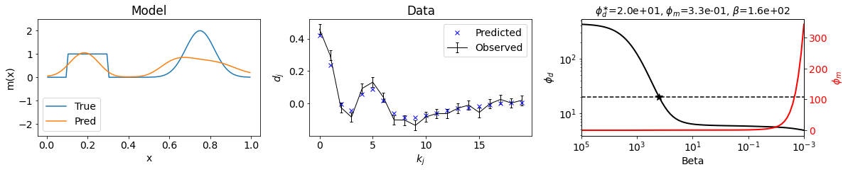
Figure E: Inversion simulation results using the model (2.3. Forward Problem-Figure A) and data (2.3. Forward Problem-Figure D) created in the Forward process above. The first panel displays the true model and recovered model from the inversion. The second panel shows both the observed (noisy) data and predicted data from the inversion. The third panel displays the data misfit and model norm terms as function of the trade-off parameter β, having run a suit of inversions with different values $\beta_k$, the optimal $\beta^*$ value indicated by the star. LinearTikhonovInversion_Notebook.ipynb

If β is too large, the model $\mathbf{m}$ is underfitting the data, causing loss of structural information.

If β is too small, the model $\mathbf{m}$ is overfitting the data, causing noise to be imaged as structure.

If β is just right $(\phi^*_d \simeq N)$, the model $\mathbf{m}$ optimally fits the data, producing the best estimate to adequately recreate the observations as was shown in Figure E.